Climate Downscaling with a ResNet

General Circulation Models (GCMs) and reanalysis products such as ERA5 represent the climate system on computational grids whose spatial resolution is insufficient for most regional applications. A single ERA5 grid cell at 0.25° spans roughly 25 km at mid-latitudes; coarser model output at 5.625° spans approximately 625 km, smoothing over orographic gradients, coastal effects, and urban heat islands that govern local climate. Re-running a GCM at higher resolution is computationally prohibitive. Statistical downscaling offers an alternative: learn a mapping from coarse to fine resolution directly from historical reanalysis data, then apply it to model output at inference cost only.

This project frames downscaling as a spatial super-resolution problem and applies a residual convolutional neural network (ResNet) to it, training on ERA5 2m temperature and evaluating against held-out high-resolution ground truth.

Overview

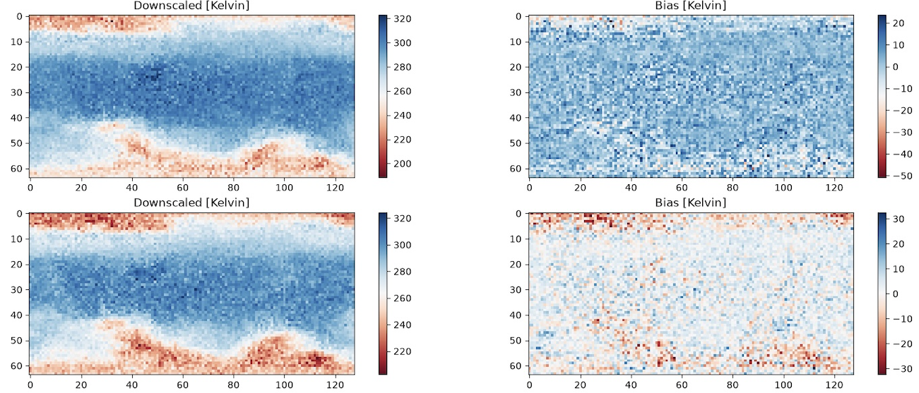
Statistical downscaling reframes an expensive re-simulation problem as supervised image super-resolution. Once trained on historical reanalysis, the network produces high-resolution temperature fields at a fraction of the cost of re-running the underlying physical model.

Background

General Circulation Models produce coarse-resolution projections of future climate. Statistical downscaling, learning high-res = f(low-res) from historical reanalysis data, is a much cheaper route to regionally actionable detail than re-running the underlying physical model at higher resolution. This project frames downscaling as an image super-resolution problem and applies CNN architectures to it.

Methodology

Data Sources

• ERA5 2m temperature (WeatherBench)
• WeatherBench benchmark paper (Rasp et al. 2020)

Approach

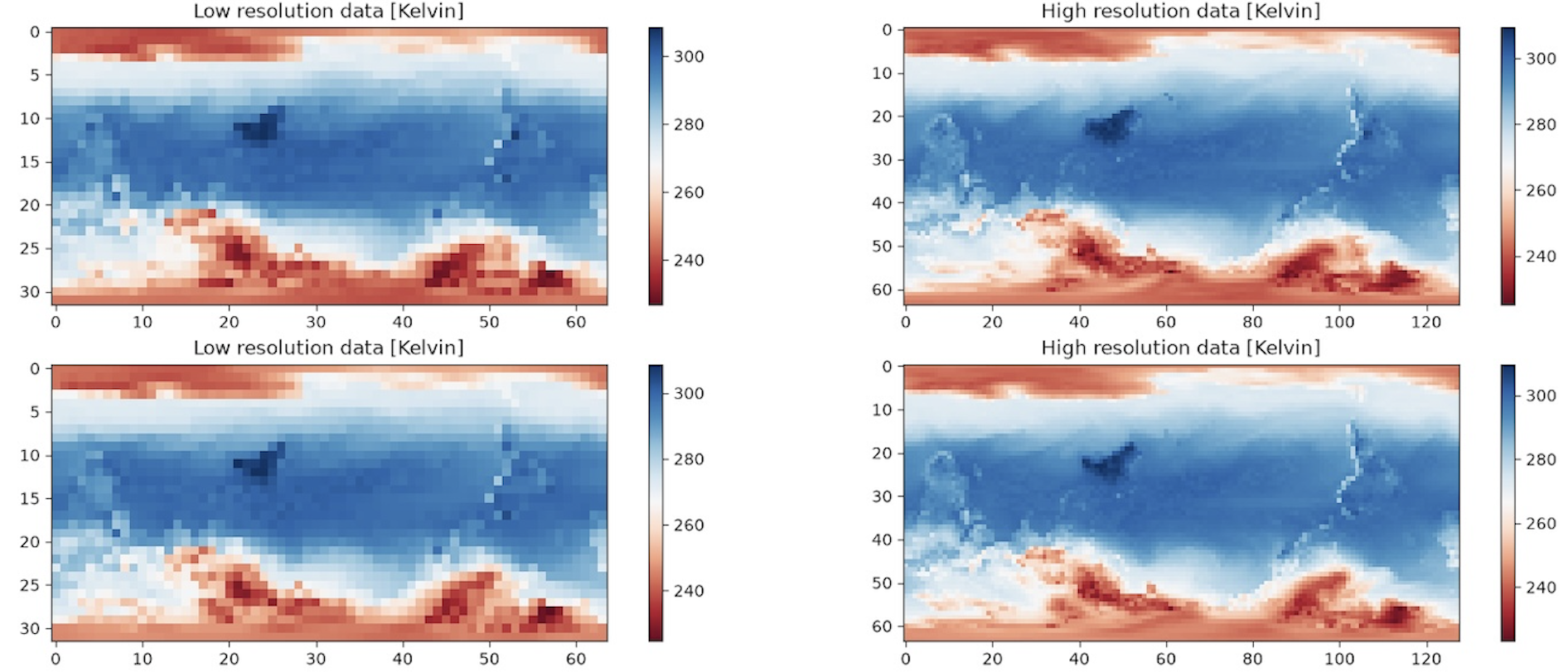
ERA5 2m temperature was degraded from its native 2.8125° to 5.625° resolution to serve as the low-resolution input, giving a 2× upscaling task on a 32×64 → 64×128 grid. A bilinear upscale of the coarsened input to the target resolution provided a smooth baseline; a ResNet backbone of 28 residual blocks with 128 hidden channels then refined this estimate, learning to recover fine-scale spatial structure that bilinear interpolation cannot reproduce. The network was optimised with MSE loss using AdamW (lr 1×10⁻⁵) under a linear warmup followed by cosine annealing.

Training was restricted to 1979 (train), 1980 (validation), and 1981–1982 (test) at daily temporal resolution - a practical adaptation to Apple Silicon hardware, where a single forward–backward pass at this model scale requires 10–25 s per batch. The full ERA5 archive (1979–2018, 6-hourly) would require approximately one day per epoch on the same hardware; the scoped run completed in a few hours.

Limitations

1. Abbreviated training period (one year of training data): the network has limited exposure to the diversity of synoptic regimes in the full ERA5 archive. Results would improve substantially with the full historical range on GPU-equipped hardware.
2. Univariate conditioning on 2m temperature only. No auxiliary predictors (topographic elevation, near-surface wind components, soil moisture) that resolve fine-scale temperature gradients in complex terrain.
3. No uncertainty quantification; the model outputs a deterministic point prediction at each grid cell.

Results

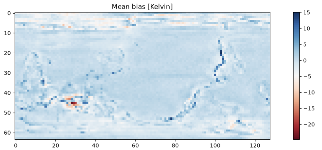
Evaluated on the 1981–1982 test period, the ResNet achieved a Pearson correlation of 0.989 against the held-out high-resolution ground truth, an RMSE of 3.64 K, and a mean bias of −1.57 K, a modest but systematic cold bias. Most errors remain within ±5 K across the test domain, with localised positive excursions in regions of high orographic complexity where statistical methods typically underperform relative to dynamical downscaling.

A ResNet trained on three years of ERA5 on consumer hardware achieves a test Pearson correlation of 0.989 against the high-resolution ground truth. The principal constraint is compute, not methodology. Extending training to the full historical record on GPU-equipped infrastructure would likely yield substantially improved spatial fidelity.

What I Learned

The notable lesson was about compute budgeting on a laptop. An early run spent 21 hours making zero epoch progress, which turned out to be a genuine arithmetic artefact (per-batch time × batches/epoch) rather than a bug. Once timed properly, scaling the dataset to match the actual hardware made the difference, with a 5-epoch run completing in a few hours. Checkpointing after every epoch (rather than only at the end) also turned out to matter in practice - a couple of training runs were killed mid-flight.